Computer vision: image recognition and processing with OpenCV

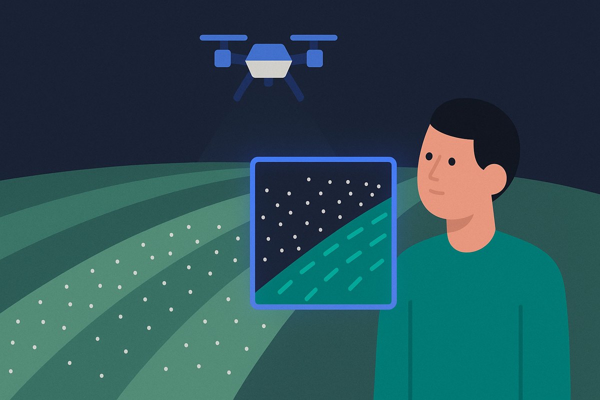
An agrotech company supplies drones for agriculture. One of its customers needed to see, from the air, whether granular fertiliser had landed evenly and which parts of the field had been left short.

Goal

The goal of the pilot was a check on fertiliser coverage, not a general crop-health model. From the drone video, the system had to show two things:

• whether the granules were spread evenly across the frame;
• where the coverage was thin, so those areas could be treated again.

Situation

The company already flew the drones and collected the video. What was missing was an analysis step on that stream. A person watching the footage could not reliably judge density or gaps, especially once the flight covered more than a small plot.

The pilot was limited on purpose. It covered one fertiliser type: granules of a known size, about 2.5-3 mm across, and visually distinct from the soil (in the test set, blue pellets). A fixed size gave the frame a scale. A distinct colour made the granules separable from the ground. Other fertilisers, liquids, and live map products were outside this pilot.

Task

For each frame of the video stream:

1. Find the granules.
2. Reject marks that are too small or too large to be that fertiliser.
3. Turn pixel size into metres, using the known granule diameter.
4. Compute density (granules per square metre).
5. Compute evenness, so a tight clump is not mistaken for good coverage.
6. Leave a result that can point at areas with too few granules.

The rest of this case is how that frame was processed with OpenCV. A video stream is a sequence of frames, so the detector runs on one frame at a time. The steps below are that detector: pre-processing, blob detection, density, and the evenness metric.

OpenCV is an open source computer vision library. It includes a large set of image and video algorithms. In this pilot the useful piece was SimpleBlobDetector, plus a colour threshold in front of it.

How a frame was processed

Each frame was a photo of soil with the blue test granules on it. The detector returned three things: the granules it found, their density, and an evenness score. Thin coverage is the frame where that score shows the granules are clumped or missing, rather than spread across the soil.

• Pre-processing image

At the beginning, we had to detect blue pellets on the image. So the first step was to make them obvious to the blob detector, which works best with contrast images with minimal noise.

A perfect result at this stage is to get a binary image of the same resolution as an original one, where pellets become white and the background becomes black. SimpleBlobDetector groups connected white pixels, so the marks have to be the light ones.

So we needed some sort of a metric to evaluate the relevance of pixel with a maximum of blue pellets and close to zero on background zones. For solving this task, we used the following formula where r, g, b correspond to red, green and blue values of each pixel [0; 255]. Take a look

relevance = max(b – (r+g)/2, 0)

0 <= relevance <= 255

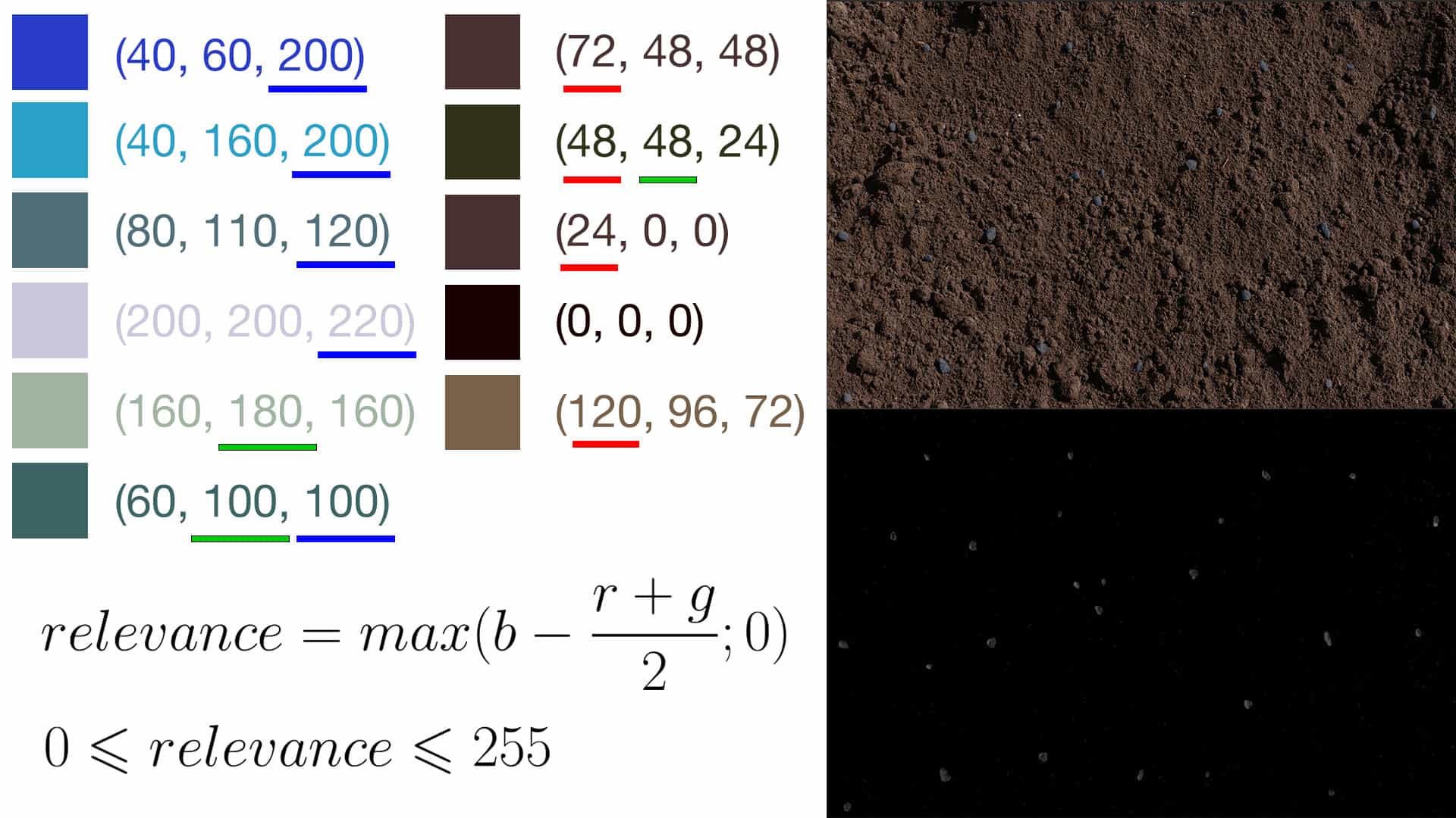
This would produce a gray image rather than a binary, but we could use a threshold function to bring the contrast up and simplify the job for a Blob Detector.

• Detect blobs

A few words of introduction. A blob is a region of an image (a group of connected pixels) shares some common properties. The main objective of blob detection methods and algorithms is to detect image regions that differ in these properties.

Here we decided to use OpenCV approach as a SimpleBlobDetector class, based on a rather simple algorithm, which includes the following steps:

• Thresholding
• Grouping
• Merging
• Center & Radius Calculation

Also, we chose this open source library for digital image processing as it ensures a convenient and simple way to detect and filter blobs based on different characteristics.

Thus, at this stage we had the following tasks to complete (correspond to the four steps mention above):

• Convert a source image to binary images by using thresholding with several thresholds
• Extract connected components from the binary images by finding Contours and defining their centers
• Group these centers from several binary images with the help of their coordinates. Then to close them (centers) form one group that corresponds to one blob
• Evaluate the final blobs' centers and their radiuses, and return as locations and sizes of the key points.

This step is pretty simple since the algorithm is implemented in SimpleBlobDetector class (OpenCV), so everything we had to do there is to set appropriate parameters.

There is an option to filter blobs by area, color, the ratio of the minimum inertia to a maximum one, convexity, and circularity. We turned off all these filters except area to handle some possible noise, which is usually less than 4 pixels.

The pellets had approximately the same size and if some too small or large blobs would be detected, we should exclude them. We made that with the help of additional filtering average values.

First, we calculated an average blob size and those values that didn't belong to [0.3 * average; 2 * average] interval were excluded.

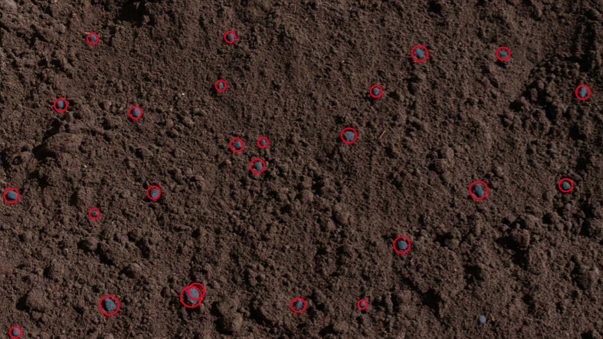
The result of this stage:

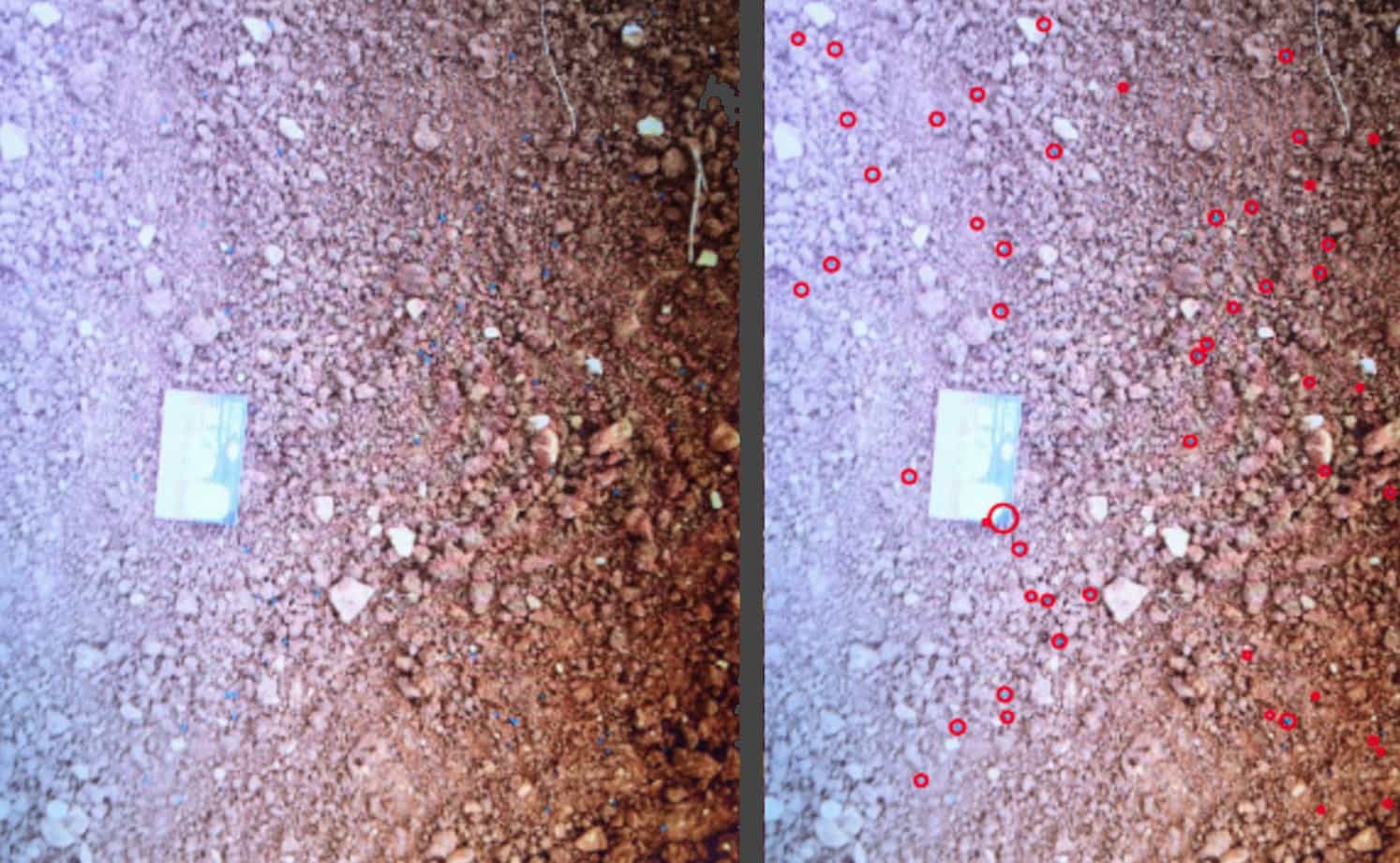
Here is another a real-world example, where we tested 10 blue paper pieces in a flower pot instead of pellets on the soil. All papers were detected perfectly, though this was a rather simple task since there were much bluer in relevant zones than in the rest of the image.

• Density

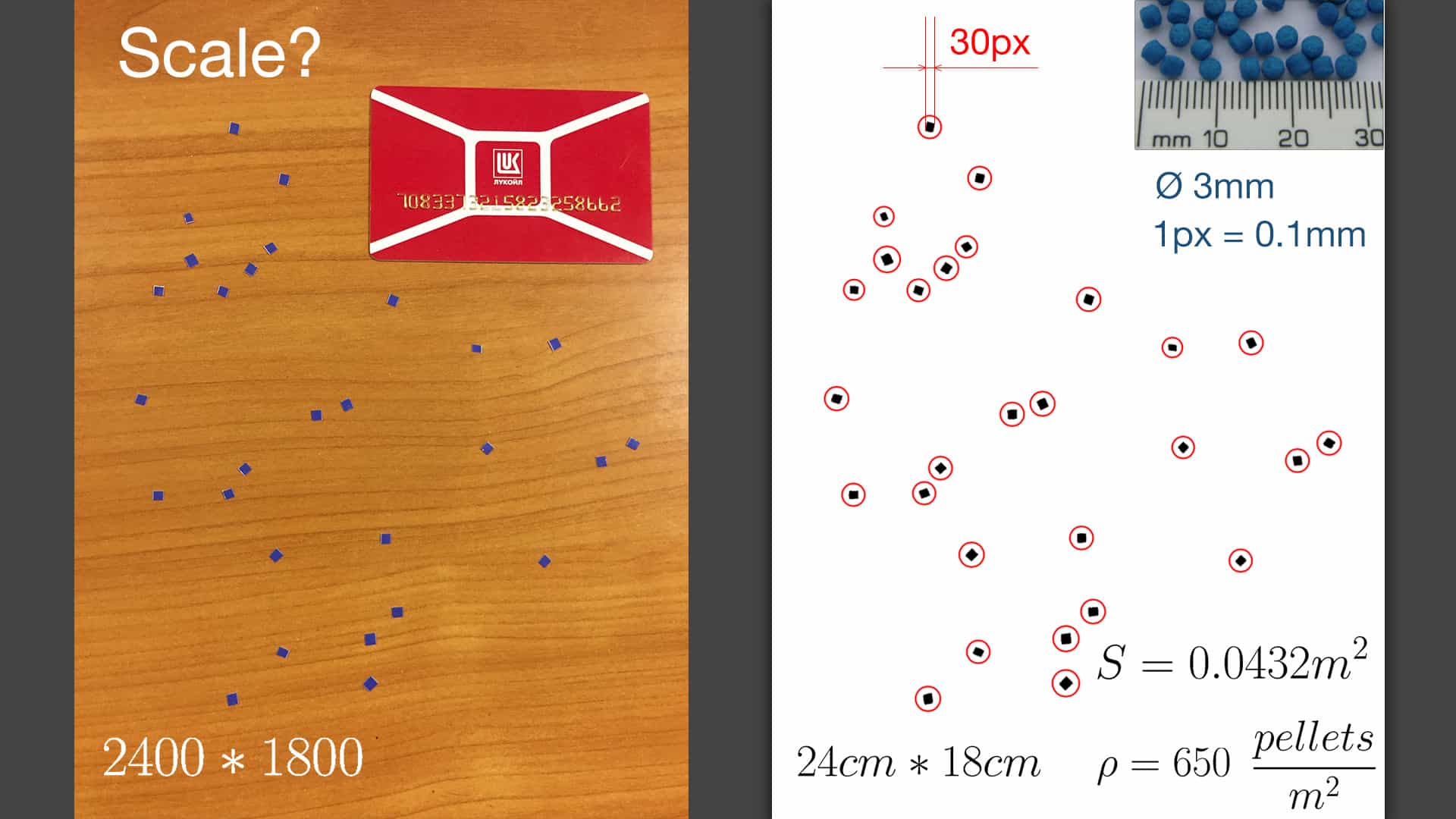
The next step was to calculate density, so we needed to know the number of pellets and the area of image in square meters: density = N/A

How could we know the real area of the image?

Well, we knew that pellets had a diameter of 2.5-3mm, and from the previous stage we knew the average size of detected blobs. So we could calculate the scale of the image and thus convert a width and height from pixels to meters. Take a look:

• Evenness (uniformity)

So, we knew the coordinates and radiuses of detected pellets as well as their density, but from a practical point of view, distribution quality depends on its evenness as much as it depends on its density.

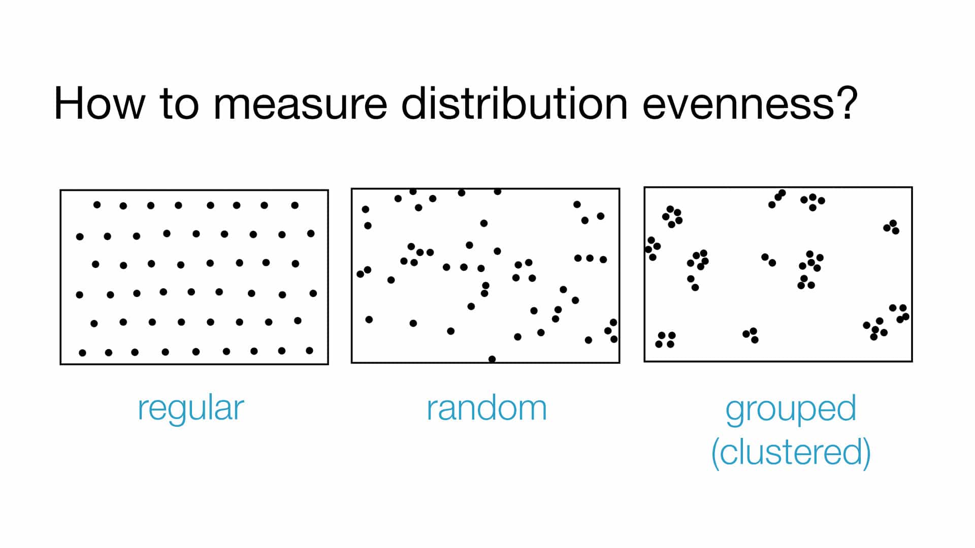
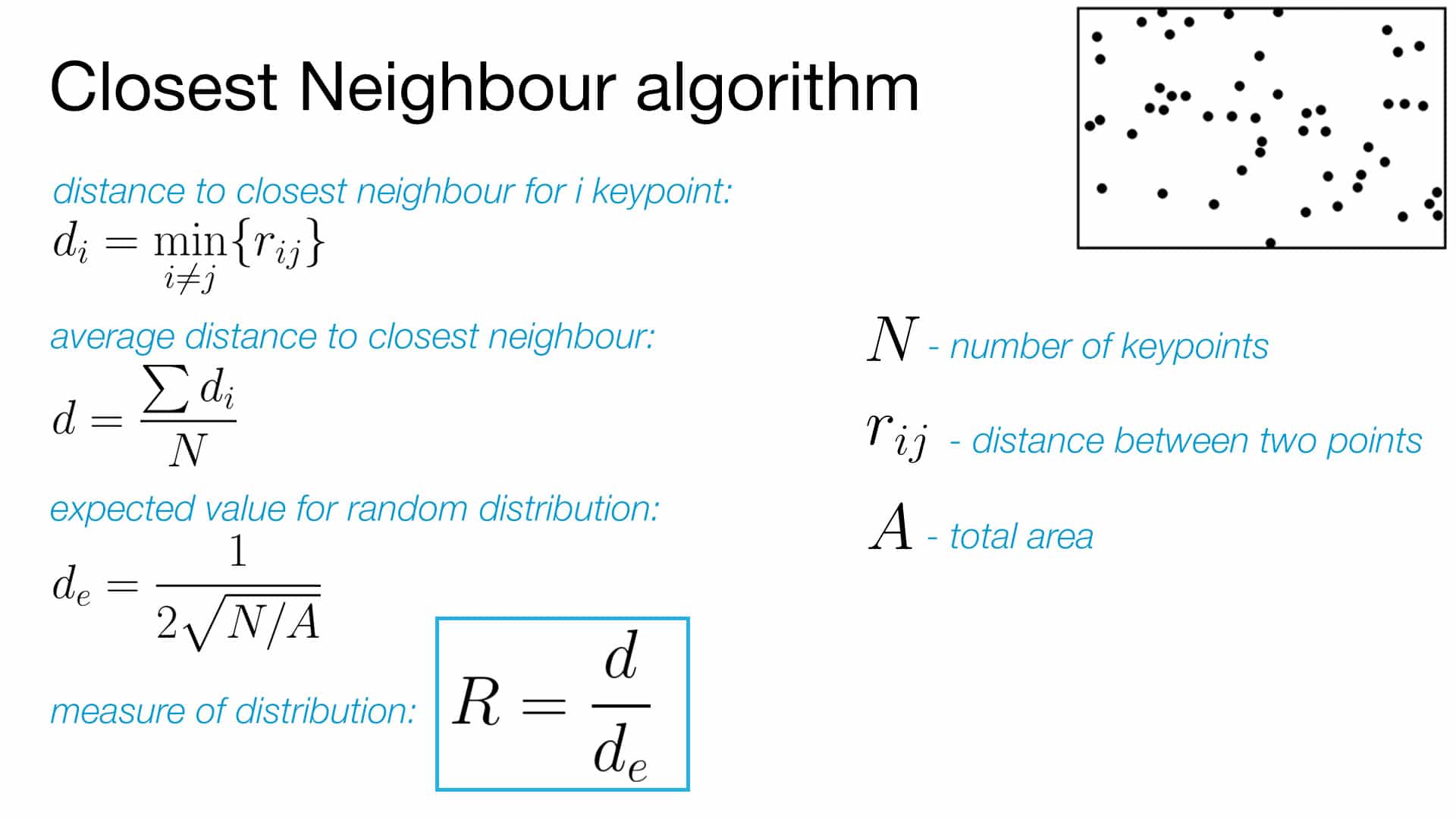
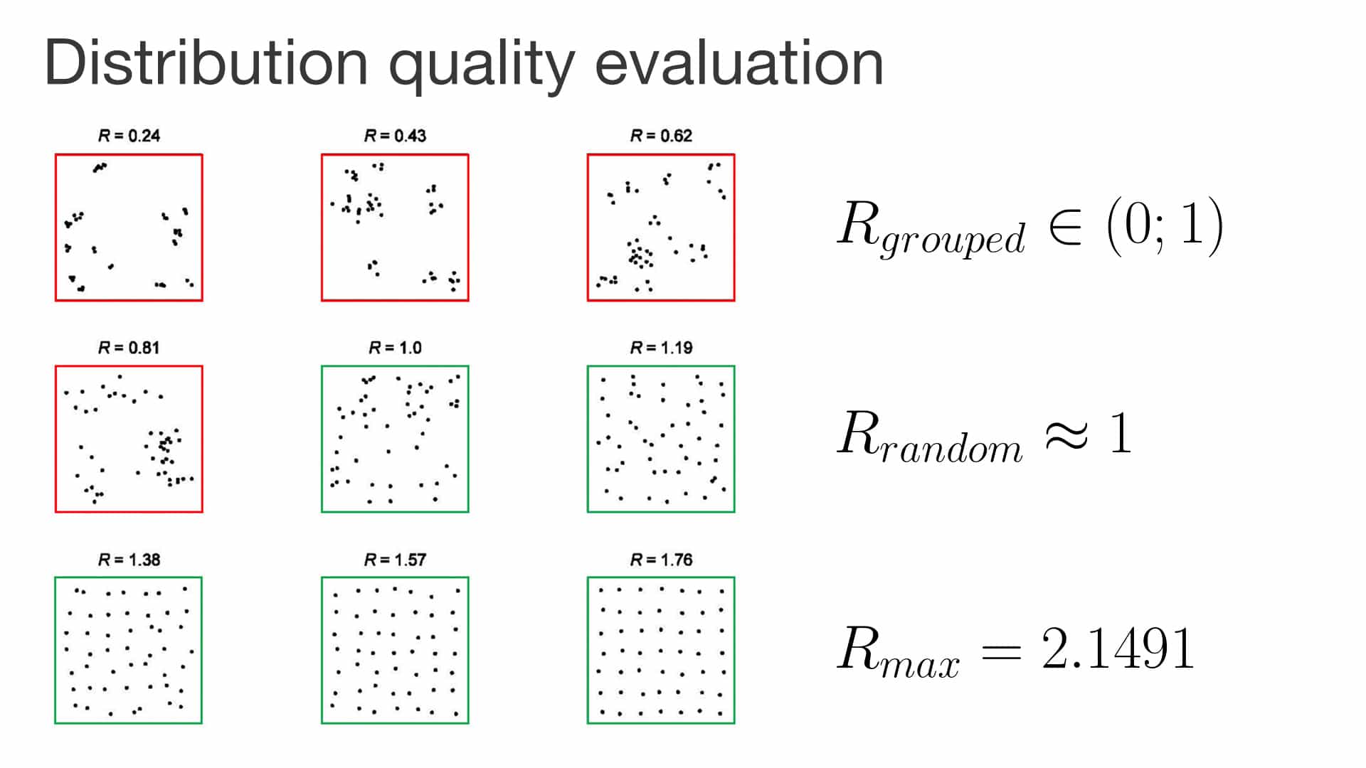
We needed a metric that is close to 0 when pellets sit in a tight group, close to 1 when they are scattered at random, and close to 2.1491 when they are spaced evenly. For that purpose, we used the closest-neighbour index (Clark and Evans, 1954) to:

• Find a distance to the closest neighbor for each point
• Calculate average of the values from the first step
• Calculate expected value for random distribution: 1/(2*sqrt(N/A))
• Divide result from step 2 by the result of step 3

On an infinite plane the index runs from 0, when every point occupies the same spot, to about 2.1491 for an even hexagonal spacing. A value near 1 is a random scatter, not an even one. On a finite photo, with no correction for the edge, the number can sit a little above 2.1491.

The detector was implemented in C++ on top of OpenCV.

Related services

• Custom software development for the processing pipeline around OpenCV
• Get in touch